Setup
Loading the R libraries and data set.
Show code
    Downloading file 1 of 2: `raw_bechdel.csv`
    Downloading file 2 of 2: `movies.csv`
Illustrating the change in Bechdel Test results over time
The first graph we want to create is an animation showing the change in Bechdel Test results over time. This animation shows the percentage of films each year (from 1940 to 2020) that meet different criteria of the Bechdel Test.
# Changing "rating" from a character to a factor variable
tt$raw_bechdel$rating <- as.factor(tt$raw_bechdel$rating)

# Levels of the "rating" variable
levels(tt$raw_bechdel$rating)
[1] "0" "1" "2" "3"# Renaming the levels of the "rating" variable
levels(tt$raw_bechdel$rating) <- c("Unscored", "It has two women...",
"...who talk to each other...",
"...about something besides a man")
# Counting the number of films with each Bechdel test rating per year
ratings_by_year <- tt$raw_bechdel %>%
group_by(year) %>%
count(year, rating)
# Counting the total number of films in each year
film_count_by_year <- ratings_by_year %>%
group_by(year) %>%
summarise(total = sum(n))
# Adding the annual film count to the Bechdel test rating count per year
ratings_by_year <- left_join(ratings_by_year, film_count_by_year)
rmarkdown::paged_table(ratings_by_year)
# Changing "year" to an integer variable
ratings_by_year$year <- as.integer(ratings_by_year$year)

# Creating an animation summarising the Bechdel test results from 1940 to 2020
p <- ratings_by_year %>%
  ggplot(aes(x = fct_rev(rating), y = (n/total), group = rating, fill = rating)) +
  geom_bar(stat = "identity") +
  scale_y_continuous(labels = scales::percent_format(scale = 100)) +
  coord_flip() +
  theme_bw() +
  theme(legend.position = "none") +
  transition_time(year, range = c(1940L, 2020L)) +
  labs(x = "Bechdel Test result", y = "Percentage of films",
       subtitle = "Year: {frame_time}",
       title = "Bechdel Test results over time") +
  ease_aes("cubic-in-out")

# Rendering the animation as a .gif
animate(p, nframes = 400, fps = 20, renderer = magick_renderer())
Figure 1: The percentage of films released each year with various Bechdel test results
Plotting the directors most likely to pass/fail the Bechdel Test
In this section, a plot is produced that shows the directors most likely to pass/fail the Bechdel Test. This is done by…
- taking all the directors in
tt$moviesas a corpus - splitting that corpus into two documents: Bechdel Test passes and failures
- calculating tf-idf to find significant directors in each document
# Selecting directors and their Bechdel pass/fail results
results_by_director <- tt$movies %>%
  select(director, binary) %>%
  filter(!is.na(director)) %>%
  separate_rows(director, sep = ", ")

# Changing "binary" to a factor variable
results_by_director$binary <- as.factor(results_by_director$binary)

# Renaming the levels of the "binary" factor
levels(results_by_director$binary) <- c("Bechdel Test Failed",
                                        "Bechdel Test Passed")

# Counting the number of times each director passes/fails the Bechdel test
results_by_director <- results_by_director %>%
  count(binary, director, sort = TRUE)

# Counting the number of times the Bechdel test has been passed/failed
total_results <- results_by_director %>%
  group_by(binary) %>%
  summarise(total = sum(n))

# Adding the total Bechdel result counts to "results_by_director"
results_by_director <- left_join(results_by_director, total_results)

# Adding tf-idf values to "results_by_director"
results_by_director <- results_by_director %>%
  bind_tf_idf(director, binary, n)

rmarkdown::paged_table(results_by_director)
# Plotting the directors with the highest tf-idf values based on Bechdel
# test results
results_by_director %>%
  group_by(binary) %>%
  slice_max(tf_idf, n = 10) %>%
  ungroup() %>%
  ggplot(aes(tf_idf, fct_reorder(director, tf-idf), fill = binary)) +
  geom_col(show.legend = FALSE) +
  facet_wrap(~binary, ncol = 2, scales = "free") +
  labs(x = "term frequency–inverse document frequency (tf-idf)", y = NULL) +
  labs(title = "Directors most likely to Pass/Fail the Bechdel Test") +
  theme_bw()
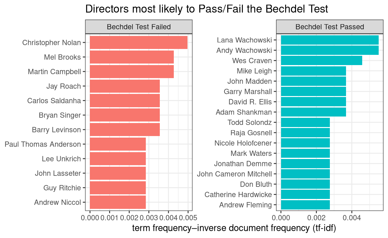
Figure 2: Directors most likely to produce films that pass/fail the Bechdel test
Plotting the writers most likely to pass/fail the Bechdel Test
In this section, the same process as the previous section is applied to the writers in tt$movies to find who is most likely to write for a film that passes/fails the Bechdel Test.
Show code
# Selecting writers and their Bechdel pass/fail results
results_by_writer <- tt$movies %>%
  select(writer, binary) %>%
  filter(!is.na(writer)) %>%
  filter(!writer == "N/A") %>%
  mutate(writer = str_remove(writer, " \\(.*")) %>%
  separate_rows(writer, sep = ", ")

# Changing "binary" to a factor variable
results_by_writer$binary <- as.factor(results_by_writer$binary)

# Renaming the levels of the "binary" factor
levels(results_by_writer$binary) <- c("Bechdel Test Failed",
                                      "Bechdel Test Passed")

# Counting the number of times each writer passes/fails the Bechdel test
results_by_writer <- results_by_writer %>%
  count(binary, writer, sort = TRUE)

# Counting the number of times the Bechdel test has been passed/failed
total_results <- results_by_writer %>%
  group_by(binary) %>%
  summarise(total = sum(n))

# Adding the total Bechdel result counts to "results_by_writer"
results_by_writer <- left_join(results_by_writer, total_results)

# Adding tf-idf values to "results_by_director"
results_by_writer <- results_by_writer %>%
  bind_tf_idf(writer, binary, n)

rmarkdown::paged_table(results_by_writer)
Show code
# Plotting the directors with the highest tf-idf values based on Bechdel
# test results
results_by_writer %>%
  group_by(binary) %>%
  slice_max(tf_idf, n = 10) %>%
  ungroup() %>%
  ggplot(aes(tf_idf, fct_reorder(writer, tf-idf), fill = binary)) +
  geom_col(show.legend = FALSE) +
  facet_wrap(~binary, ncol = 2, scales = "free") +
  labs(x = "term frequency–inverse document frequency (tf-idf)", y = NULL) +
  labs(title = "Writers most likely to Pass/Fail the Bechdel Test") +
  theme_bw()
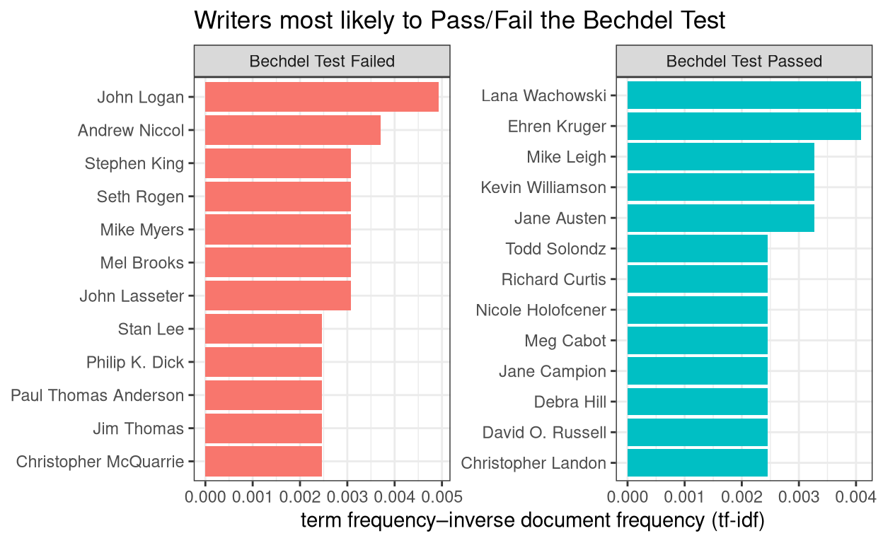
Figure 3: Writers most likely to produce films that pass/fail the Bechdel test