Summary
In this post, a machine learning model is created using this week’s #TidyTuesday data set: CEO Departures. This data set contains descriptions of thousands of CEO departures and reasons for these departures. After filtering missing values from the data set and simplifying the departure reasons to “Voluntary” and “Involuntary”, a machine learning model is trained to distinguish between these departure categories. The model used is a linear support-vector machine (SVM) instructed to categorise departures based on individual words used in the departure descriptions. The final model is limited by class imbalance in the data set, as most of the CEO departures were voluntary.
Setup
Show code
# Loading libraries
library(tidyverse)
library(tidytuesdayR)
library(tidymodels)
library(textrecipes)
library(themis)
library(parsnip)
library(doParallel)

# Installing the GitHub version of {parsnip} to use svm_linear()
#devtools::install_github("tidymodels/parsnip")

# Loading data set
tt <- tt_load("2021-04-27")
Downloading file 1 of 1: `departures.csv`Data wrangling
Wrangling data for machine learning and visualisation.
Show code
# Creating a new variable "depart_vol" to record CEO departures as
## Voluntary or Involuntary
departures <- tt$departures %>% mutate(depart_vol = factor(departure_code))
# Setting descriptive factor levels for "depart_vol"
levels(departures$depart_vol) <- list(
  "Involuntary" = levels(departures$depart_vol)[1:4],
  "Voluntary" = levels(departures$depart_vol)[5:6],
  "Other" = levels(departures$depart_vol)[7:9]
  )

# Filtering "depart_vol" and "notes" to a new object: "depart_notes"
depart_notes <- departures %>%
  filter(!is.na(notes) & !is.na(depart_vol)) %>%
  filter(depart_vol != "Other") %>%
  select(depart_vol, notes)

# Dropping empty factor levels. In this case, the level "Other" is empty
depart_notes$depart_vol <- droplevels(depart_notes$depart_vol)
# Printing the number of Involuntary and Voluntary CEO departures with descriptions
table(depart_notes$depart_vol)
Involuntary   Voluntary
       1694        3771
Setting parameters for machine learning model
In this section…
- The filtered data set is split into training and test data
- 10-fold cross-validation (CV) is set for the training subset to get a more accurate estimate of training performance
- Feature engineering parameters are set
- The linear SVM model parameters are set
- Feature engineering and model parameters are combined into a workflow
- Performance metrics are selected
Show code
# Setting seed for reproducibility
set.seed(100)
# Splitting depart_notes into training and test data
departures_split <- depart_notes %>%
  initial_split(strata = depart_vol)

# Creating training and test sets using departures_split
departures_train <- training(departures_split)
departures_test <- testing(departures_split)

# Setting seed for reproducibility
set.seed(100)
# Setting 10-fold cross-validation (CV) using training data
departures_folds <- vfold_cv(departures_train, strata = depart_vol)
# Printing 10-fold CV splits
departures_folds
#  10-fold cross-validation using stratification
# A tibble: 10 x 2
   splits             id
   <list>             <chr>
 1 <split [3688/410]> Fold01
 2 <split [3688/410]> Fold02
 3 <split [3688/410]> Fold03
 4 <split [3688/410]> Fold04
 5 <split [3688/410]> Fold05
 6 <split [3688/410]> Fold06
 7 <split [3688/410]> Fold07
 8 <split [3688/410]> Fold08
 9 <split [3689/409]> Fold09
10 <split [3689/409]> Fold10
Show code
# Feature engineering
## Creating preprocessing recipe for predicting voluntary/involuntary departures
departures_rec <-  recipe(depart_vol ~ notes, data = departures_train) %>%
  # Splitting the "notes" variable into individual tokens (words)
  step_tokenize(notes) %>%
  # Limiting number of tokens used in model
  step_tokenfilter(notes, max_tokens = 1000) %>%
  # Weighing tokens by tf-idf
  step_tfidf(notes) %>%
  # Normalising numeric predictors
  step_normalize(all_numeric_predictors()) %>%
  # Upsampling to address class imbalance
  step_smote(depart_vol)

# Specifying the machine learning model
## This model will use a linear Support Vector Machine (SVM)
svm_spec <- svm_linear() %>%
  set_mode("classification") %>%
  set_engine("LiblineaR")

# Combining the feature engineering recipe and model spec to create a workflow
departures_wf <- workflow() %>%
  add_recipe(departures_rec) %>%
  add_model(svm_spec)
# Printing the workflow
departures_wf
══ Workflow ══════════════════════════════════════════════════════════
Preprocessor: Recipe
Model: svm_linear()

── Preprocessor ──────────────────────────────────────────────────────
5 Recipe Steps

• step_tokenize()
• step_tokenfilter()
• step_tfidf()
• step_normalize()
• step_smote()

── Model ─────────────────────────────────────────────────────────────
Linear Support Vector Machine Specification (classification)

Computational engine: LiblineaR
Show code
# Selecting the metrics used for modelling
departures_metrics <- metric_set(accuracy, recall, precision)
Creating a model using the training subset
In this section, a linear SVM model is created using the training subset with 10-fold CV.
Show code
# Setting up parallel processing
cl <- makePSOCKcluster(detectCores() - 1)
registerDoParallel(cl)

# Setting seed for reproducibility
set.seed(100)
# Fitting models using resampling
svm_results <- fit_resamples(
  departures_wf, # Specifying workflow
  departures_folds, # Specifying cross validation folds
  metrics = departures_metrics, # Metrics used for modelling
  control = control_resamples(save_pred = TRUE) # Saving predictions for confusion matrix
)

# Printing performance metrics of SVM model
collect_metrics(svm_results)
# A tibble: 3 x 6
  .metric   .estimator  mean     n std_err .config
  <chr>     <chr>      <dbl> <int>   <dbl> <chr>
1 accuracy  binary     0.804    10 0.00592 Preprocessor1_Model1
2 precision binary     0.677    10 0.0102  Preprocessor1_Model1
3 recall    binary     0.706    10 0.00925 Preprocessor1_Model1
Creating a model using the full data set
In this section, the final linear SVM model is created using the full data set.
Show code
# Setting seed for reproducibility
set.seed(100)

# Fitting the final model
final_fitted <- last_fit(departures_wf, departures_split,
                      metrics = departures_metrics)

# Printing performance metrics of final fitted model
collect_metrics(final_fitted)
# A tibble: 3 x 4
  .metric   .estimator .estimate .config
  <chr>     <chr>          <dbl> <chr>
1 accuracy  binary         0.813 Preprocessor1_Model1
2 recall    binary         0.708 Preprocessor1_Model1
3 precision binary         0.694 Preprocessor1_Model1
Confusion matrices for training and full models
In this section, confusion matrices are printed for the linear SVM models created using the training subset and full data set. The confusion matrix for the final model is plotted to illustrate the differences between this model’s predictions and the true values in the data set. From this plot, we can see that there is a class imbalance in the data set: most of the CEO departures with descriptions were Voluntary. As a result, Voluntary CEO departures are more accurately predicted based on event descriptions than Involuntary departures. Class imbalances can be addressed by upsampling (creating new examples of the minority class), which is used in the feature engineering of this model. Ideally, this data set would have more descriptions of Involuntary CEO departures.
Show code
# Printing the confusion matrix of the model trained using the 10-fold cv
## training data
svm_results %>%
  conf_mat_resampled(tidy = FALSE)
            Involuntary Voluntary
Involuntary        89.7      42.9
Voluntary          37.3     239.9
Show code
# Printing the confusion matrix of the final fitted model
collect_predictions(final_fitted) %>%
  conf_mat(depart_vol, .pred_class)
             Truth
Prediction    Involuntary Voluntary
  Involuntary         300       132
  Voluntary           124       811
Show code
# Visualising confusion matrix of the final fitted model
collect_predictions(final_fitted) %>%
  conf_mat(depart_vol, .pred_class) %>%
  autoplot() +
  labs(title = "Prediction vs Truth for final linear SVM model",
       subtitle = "Class imbalance is an issue; most of the observations were of Voluntary CEO departures")
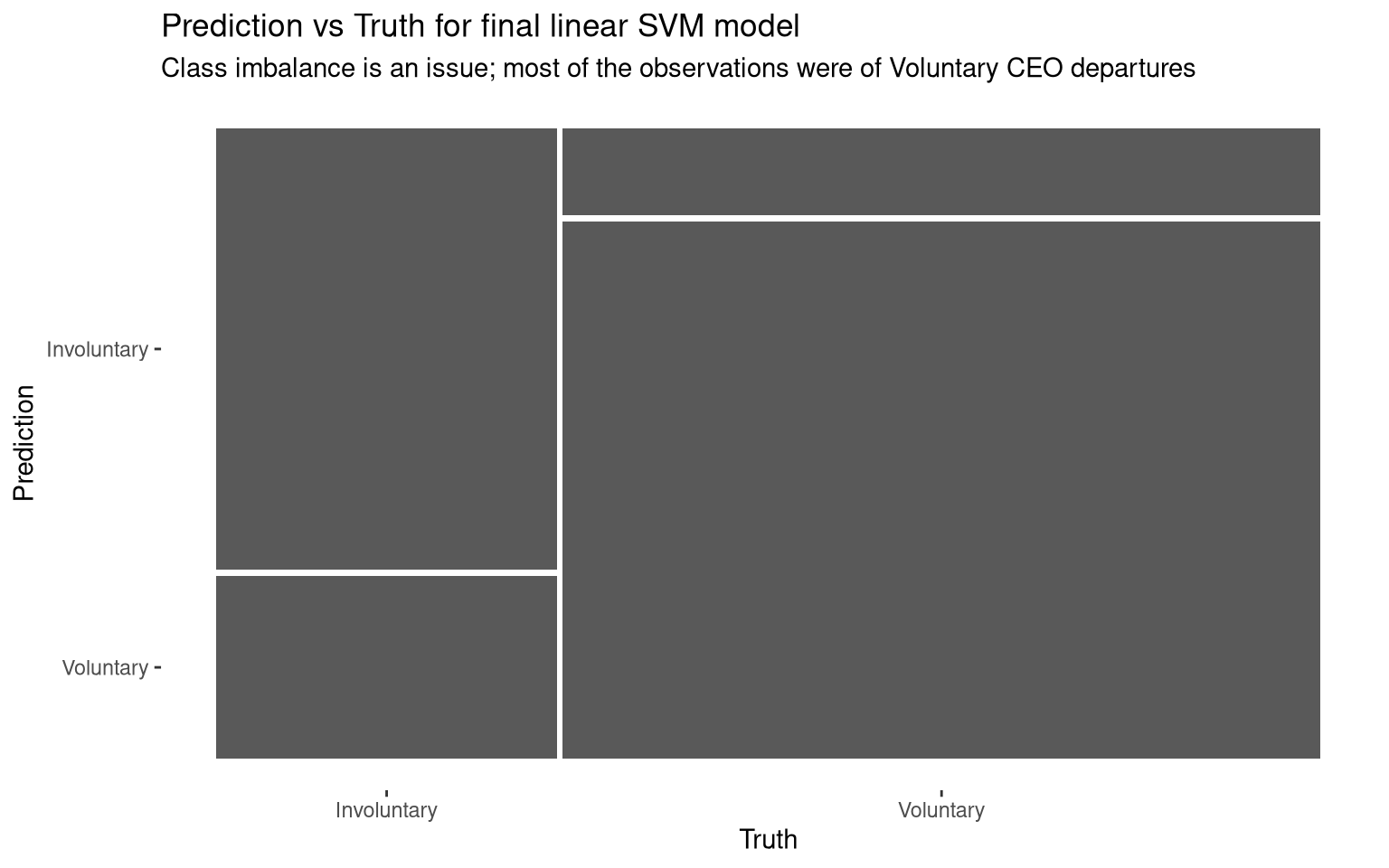
Figure 1: Confusion matrix for the final linear SVM model.
Significant words according to the final model
In this section, the most important words for predicting whether a CEO departure was Involuntary or Voluntary are visualised. This is based on the coefficients from the final linear SVM model: words with higher predictive value are given coefficients with larger absolute values.
From this plot, we can see that descriptions of Involuntary CEO departures are more likely to include the words “health”, “died”, “charge” and “dropped”. Descriptions of Voluntary CEO departures are more likely to include the words “retired”, “voluntarily”, “join” and “consulting”. Involuntary CEO departures described in the data set are likely due to poor health, death and litigation; Voluntary CEO departures are likely due to retirement, former executives joining other companies, or moving into consulting.
Show code
# Extracting model fit
departures_fit <- pull_workflow_fit(final_fitted$.workflow[[1]])

# Visualising the most important words for predicting whether a CEO departure
## was voluntary
tidy(departures_fit) %>%
  filter(term != "Bias") %>%
  group_by(sign = estimate > 0) %>%
  slice_max(abs(estimate), n = 15) %>%
  ungroup() %>%
  mutate(term = str_remove(term, "tfidf_notes_"), # Tidying terms
         sign = ifelse(sign, "More likely from Voluntary CEO departures",
                       "More likely from Involuntary CEO departures")) %>%
  ggplot(aes(abs(estimate), fct_reorder(term, abs(estimate)), fill = sign)) +
  geom_col(show.legend = FALSE) +
  facet_wrap(~sign, scales = "free") +
  labs(x = "Coefficient from linear SVM", y = NULL) +
  scale_fill_brewer(palette = "Set1") +
  theme_classic() +
  labs(titles = "Which words are more likely to be used when a CEO leaves Involuntarily vs. Voluntarily?",
       subtitle = "Importance assigned by linear SVM model, based on descriptions of CEO departures")
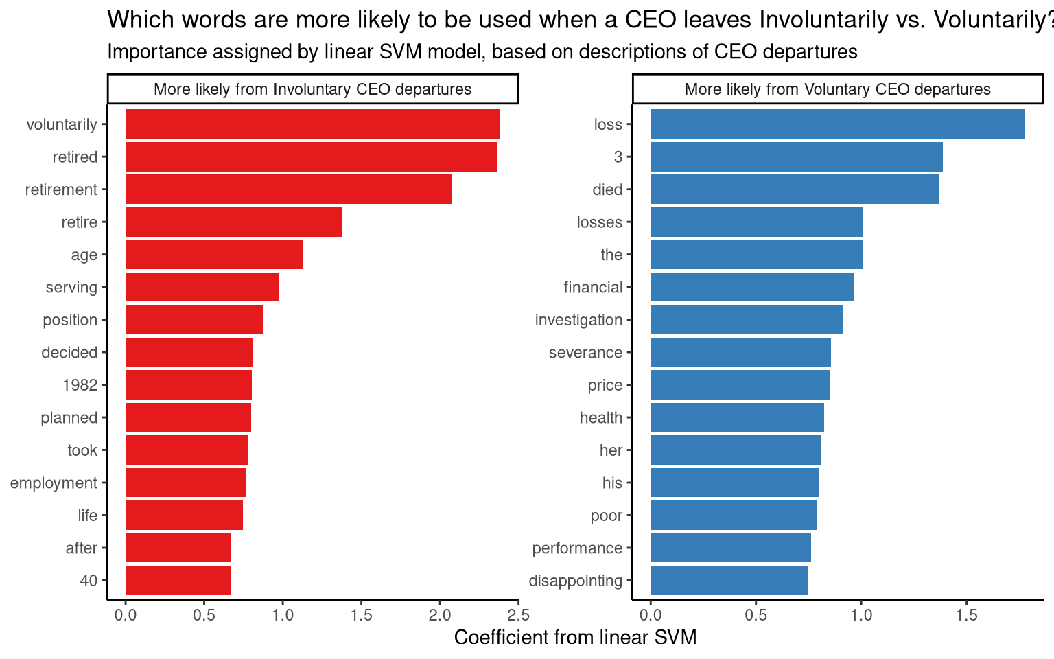
Figure 2: Words most likely to appear in CEO departure descriptions in each category, according to the linear SVM model.
References