Introduction
In this post, the BEA Infrastructure Investment data set from the #TidyTuesday project is used to illustrate variable transformation and the exploreR::masslm() function. The variable for gross infrastructure investment adjusted for inflation is transformed to make it less skewed. Using these transformed investment values, multiple linear models are then created to quickly see which variables in the data set have the largest impact on infrastructure investment.
Setup
Loading the R libraries and data set.
Show code
    Downloading file 1 of 3: `ipd.csv`
    Downloading file 2 of 3: `chain_investment.csv`
    Downloading file 3 of 3: `investment.csv`
Plotting distribution of inflation-adjusted infrastructure investments
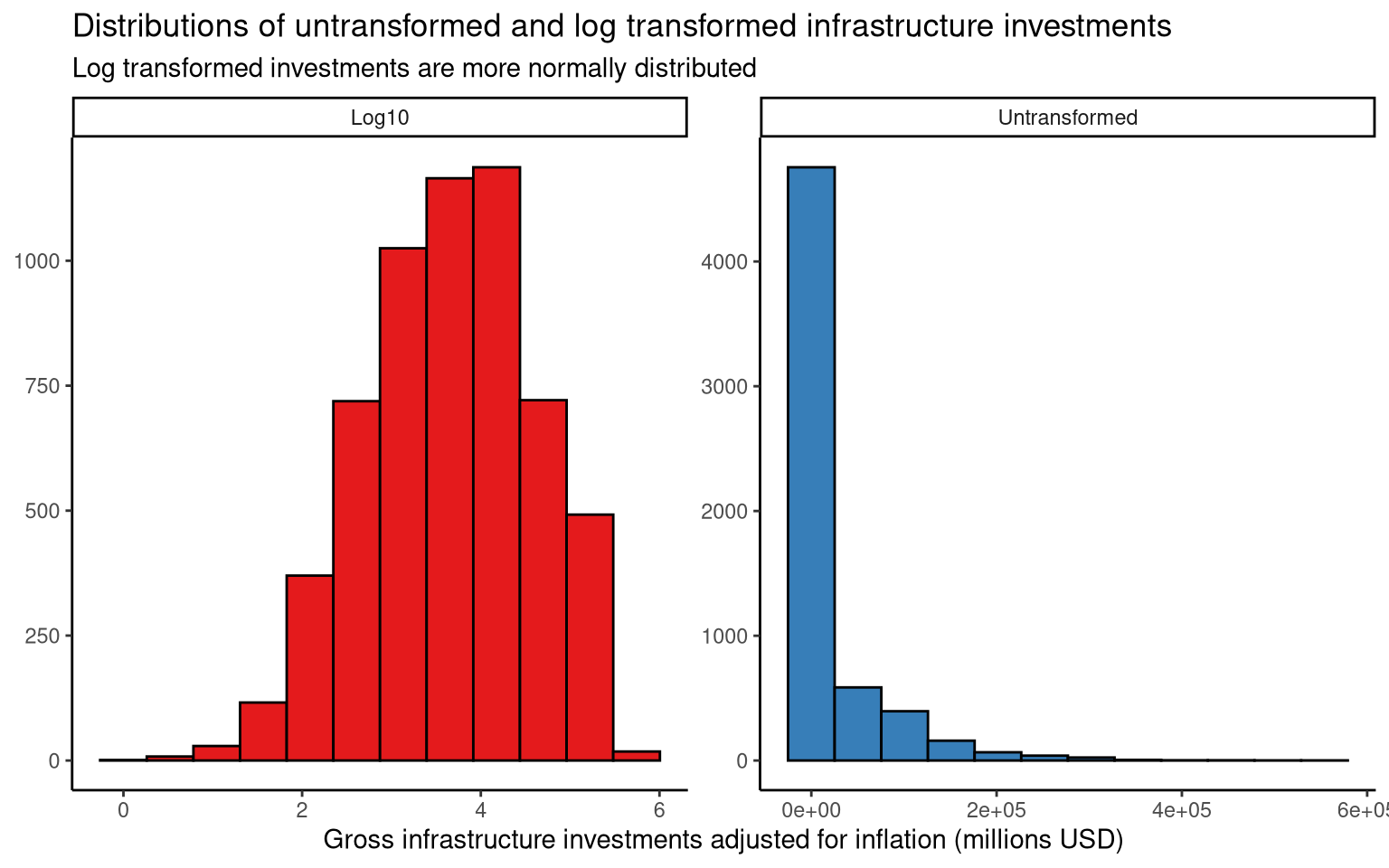
In this section, the gross infrastructure investment (chained 2021 dollars) in millions of USD are plotted with and without a \(\log{10}\) transformation. From the histograms below, we can see that applying a \(\log{10}\) transformation gives the variable a less skewed distribution. This transformation should be considered for statistical testing of inflation-adjusted infrastructure investments.
Show code
# Creating tbl_df with gross_inv_chain values
untransformed_tbl_df <- tibble(
  gross_inv_chain = tt$chain_investment$gross_inv_chain,
  transformation = "Untransformed"
  )

# Creating tbl_df with log10(gross_inv_chain) values
log10_tbl_df <- tibble(
  gross_inv_chain = log10(tt$chain_investment$gross_inv_chain),
  transformation = "Log10"
)

# Combining the above tibbles into one tbl_df
gross_inv_chain_tbl_df <- rbind(untransformed_tbl_df, log10_tbl_df)

# Plotting distribution of inflation-adjusted infrastructure investments
gross_inv_chain_tbl_df %>%
  ggplot(aes(x = gross_inv_chain, fill = transformation)) +
  geom_histogram(show.legend = FALSE, position = "identity",
                 bins = 12, colour = "black") +
  facet_wrap(~transformation, scales = "free") +
  labs(fill.position = "none", y = NULL,
       x = "Gross infrastructure investments adjusted for inflation (millions USD)",
       title = "Distributions of untransformed and log transformed infrastructure investments",
       subtitle = "Log transformed investments are more normally distributed") +
  scale_fill_brewer(palette = "Set1") +
  theme_classic()

(#fig:figure_1)The transformed variable is more appropriate for parametric statistical tests.
Exploring a data set using mass linear regression
In this section, exploreR::masslm() is applied to a copy of the data set with \(\log{10}\) transformed investment values. The masslm() function from the exploreR package quickly produces a linear model of the dependent variable and every other variable in the data set. It then returns a data frame containing the features of each linear model that are useful when selecting predictor variables:
- R squared The proportion of variation in the dependent (response) variable that is explained by the independent (predictor) variable.
- p-value The statistical significance of the model. A p-value \(\lt 5\%\) is typically considered significant.
This function is useful for quickly determining which variables should be included in predictive models. Note that the data set used should satisfy the assumptions of linear models, including a normally distributed response variable. In this case, the \(\log{10}\) transformed investment variable is close to normal.
From this mass linear regression model, we can see that investment category is the single variable that explains the largest proportion of variation in \(\log{10}\) investment; and the linear model with group number is the most significant, followed by year.
Show code
# Creating a copy of the chain_investment data set with log10 transformed
# gross investment values
chain_investment_df <- tt$chain_investment %>%
  # Creating a log10 transformed copy of gross_inv_chain
  mutate(gross_inv_transformed = log10(gross_inv_chain)) %>%
  # Removing -Inf values
  filter(gross_inv_transformed != -Inf) %>%
  # Selecting variables to include in the data frame
  select(category, meta_cat, group_num, year, gross_inv_transformed)

# Applying mass linear regression
transformed_investment_masslm <- masslm(chain_investment_df,
                                        dv.var = "gross_inv_transformed")

# Printing the masslm results in order of R squared values (decreasing)
transformed_investment_masslm %>%
  arrange(-R.squared)
         IV Coefficient    P.value  R.squared
1  category   -0.579900  8.471e-10 0.63754622
2  meta_cat    0.349300  7.848e-10 0.37782201
3 group_num   -0.058750 3.625e-204 0.14695670
4      year    0.009507  7.007e-59 0.04377399
Show code
# Printing the masslm results in order of p-values
transformed_investment_masslm %>%
  arrange(P.value)
         IV Coefficient    P.value  R.squared
1 group_num   -0.058750 3.625e-204 0.14695670
2      year    0.009507  7.007e-59 0.04377399
3  meta_cat    0.349300  7.848e-10 0.37782201
4  category   -0.579900  8.471e-10 0.63754622
References
- exploreR vignette: The How and Why of Simple Tools