Text mining Star Trek dialogue and classifying characters using machine learning

Graphs, text mining and analysis using the #TidyTuesday data set for week 34 of 2021 (17/8/2021): “Star Trek voice commands”

Introduction

In this article, the Star Trek voice commands data set from the #TidyTuesday project is used to investigate character diction using text mining, and train a machine learning model to distinguish between people and computers in the data set. The techniques used in this article are taken from the following textbooks, both of which are freely available online:

1. Text Mining with R
2. Supervised Machine Learning for Text Analysis in R

Setup

Loading the R libraries and data set.

# Loading libraries
library(tidytuesdayR) # For loading data set
library(textrecipes) # For adding tf-idf to recipies (step_tfidf)
library(tidyverse) # For the ggplot2, dplyr, forcats libraries
library(tidytext) # For text mining
library(glmnet) # For lasso model
library(tidymodels) # For various modelling libraries

# Loading data set
tt <- tt_load("2021-08-17")

    Downloading file 1 of 1: `computer.csv`

Most spoken words by prominent characters

The first graph plots the words most frequently used by prominent characters when talking to computers. They were chosen by selecting characters in the data set that appeared more than 150 times each.

# Creating a vector of characters with most interactions with computers
chars_with_most_interactions <- tt$computer %>%
  filter(char_type != "Computer") %>% # Filtering out rows for computer lines
  count(char, sort = TRUE) %>% # Counting the number of rows for each character
  filter(n >= 150) %>% # Filtering out characters with under 150 lines
  pull(char) # Pulling the names of the characters as a vector

# Counting words spoken per character
character_words <- tt$computer %>%
  filter(char %in% chars_with_most_interactions) %>% # Selecting rows
  unnest_tokens(word, interaction) %>% # Creating a row per word in interaction
  anti_join(get_stopwords(), by = "word") %>% # Removing stop words
  count(char, word, sort = TRUE) # Counting words per character

# Plotting most spoken words per character
character_words %>%
  group_by(char) %>%
  slice_max(n, n = 15, with_ties = FALSE) %>%
  ungroup() %>%
  ggplot(aes(n, fct_reorder(word, n), fill = char)) +
  geom_col(show.legend = FALSE) +
  facet_wrap(~char, ncol = 2, scales = "free") +
  scale_fill_viridis_d() +
  theme_classic() +
  labs(title = "Words most frequently spoken by prominent characters",
       x = "Utterances", y = "Words")

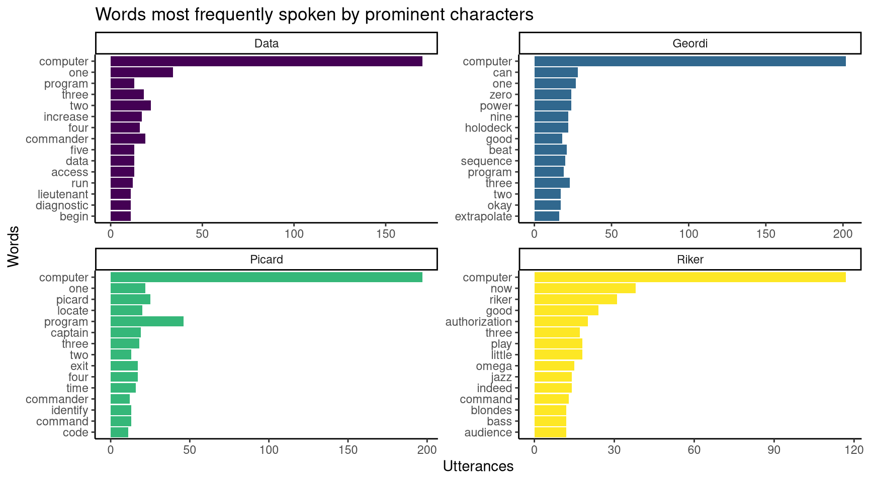
Figure 1: The most frequently spoken word is computer.

Words specific to prominent characters

From Figure 1, we can see that the most frequently spoken word across all four characters is “computer”. This is not surprising, as this data set records interactions between characters and computers, with characters addressing the computers as “computer”. An expected result, but it does not tell us anything about the characters. What if we wanted to see which words were specific to each character?

To see which words are specific to these characters, we can use term frequency-inverse document frequency (tf-idf) to measure word importance. For a given word, tf-idf increases the more often it is used, and decreases relative to the number of documents it appears in. In this case, each “document” refers to a character. So even though “computer” is the most frequent term used by the characters, it will have a low tf-idf value as it is used by every character (therefore it appears in every document).

# Counting total number of words spoken per character
total_words <- character_words %>% 
  group_by(char) %>%  # Grouping words by character
  summarize(total = sum(n)) # Counting words spoken per character ("total")

# Joining tbl_dfs: adding "total" variable to character_words
character_words <- left_join(character_words, total_words)

# Adding tf_idf to character_words
character_words <- character_words %>%
  bind_tf_idf(term = word, document = char, n = n) %>%
  arrange(desc(tf_idf)) # Arranging rows by descending tf_idf values

# Printing a summary of the character_words object
glimpse(character_words)

Rows: 1,492
Columns: 7
$ char   <chr> "Riker", "Riker", "Riker", "Riker", "Riker", "Riker",…
$ word   <chr> "little", "omega", "indeed", "jazz", "good", "audienc…
$ n      <int> 18, 15, 14, 14, 24, 12, 12, 12, 12, 12, 12, 12, 12, 1…
$ total  <int> 1144, 1144, 1144, 1144, 1144, 1144, 1144, 1144, 1144,…
$ tf     <dbl> 0.015734266, 0.013111888, 0.012237762, 0.012237762, 0…
$ idf    <dbl> 1.3862944, 1.3862944, 1.3862944, 1.3862944, 0.6931472…
$ tf_idf <dbl> 0.02181232, 0.01817694, 0.01696514, 0.01696514, 0.014…

# Plotting words with the top tf-idf values per character
character_words %>%
  group_by(char) %>%
  slice_max(tf_idf, n = 15, with_ties = FALSE) %>%
  ungroup() %>%
  ggplot(aes(tf_idf, fct_reorder(word, tf_idf), fill = char)) +
  geom_col(show.legend = FALSE) +
  facet_wrap(~char, ncol = 2, scales = "free") +
  scale_fill_viridis_d() +
  theme_classic() +
  labs(title = "Spoken words specific to each character",
       subtitle = "Words listed are used often by each character relative to other characters",
       y = "Words",
       x = "term frequency-inverse document frequency (tf-idf)")

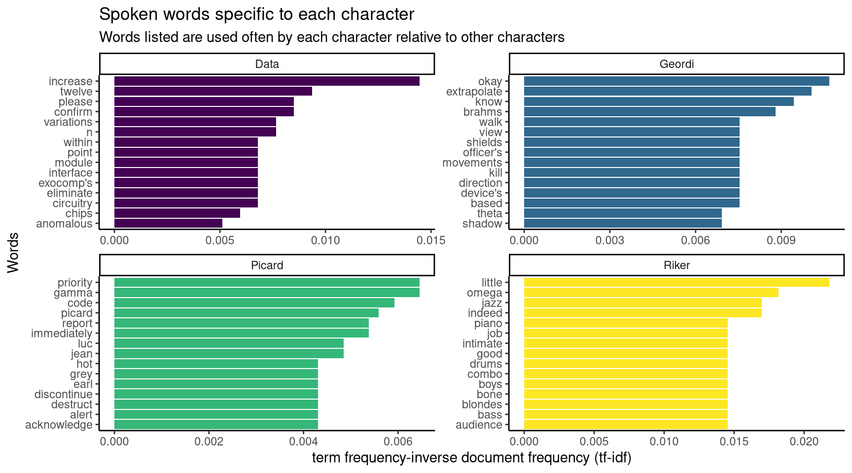
Figure 2: Data is the most likely character to say please when addressing a computer. Riker likes jazz. Picard likes to say his own name

Specifying a model to classify People and Computers in the data set

In this section, a machine learning model for classifying interactions into categories is set up. The variable “char_type” divides the data set into two categories: the lines spoken by people to computers (char_type = “Person”) and responses from the computers (char_type = “Computer”). The goal of this model is to look at the dialogue in the “interaction” variable, and determine whether that dialogue was spoken by a “Person” or “Computer” character based on the words used. To do this:

• The data set is split into a subset for training the machine learning model and a subset for testing the model
• The training data is split into ten folds, each with its own training and testing sections (10-fold cross-validation)
• A number of preprocessing steps for the data set are defined
• The type of machine learning model is defined (a lasso regularised model)
• The preprocessing steps and model type are combined into a workflow

The preprocessing for this data set includes a downsampling step. There is a class imbalance in this dataset, as there are over twice the number of “Person” interactions as “Computer” ones. Including the downsampling step addresses this class imbalance by removing observations of the majority class (“Person”) during training.

# Summarising the values in the char_type variable
tt$computer %>% select(char_type) %>% table()

.
Computer   Person 
     708     1506 

# Setting seed for reproducibility
set.seed(20210818)
# Splitting data into training and test subsets
char_type_split <- tt$computer %>%
  initial_split(strata = char_type) # Ensures equal proportion of char_type

# Creating training and test sets using departures_split
char_type_train <- training(char_type_split)
char_type_test <- testing(char_type_split)

# Setting seed for reproducibility
set.seed(20210818)
# Setting up 10-fold cross-validation (CV) using training data
char_type_folds <- vfold_cv(char_type_train,
                            strata = char_type) # Ensures equal proportion of char_type

# Creating preprocessing recipe for predicting if lines are spoken by a computer
char_type_rec <-  recipe(char_type ~ interaction, data = char_type_train) %>%
  step_tokenize(interaction) %>% # Splitting interaction variable into words
  step_tokenfilter(interaction, max_tokens = 1500) %>% # Limiting tokens used
  step_tfidf(interaction) %>% # Weighing tokens by tf-idf
  themis::step_downsample(char_type) # Downsampling to address class imbalance

# Specifying a lasso regularised model
lasso_spec <- logistic_reg(penalty = 0.01, mixture = 1) %>%
  set_mode("classification") %>%
  set_engine("glmnet")

# Creating a supervised machine learning workflow
char_type_wf <- workflow() %>%
  add_recipe(char_type_rec) %>%
  add_model(lasso_spec)

# Printing workflow
char_type_wf

══ Workflow ══════════════════════════════════════════════════════════
Preprocessor: Recipe
Model: logistic_reg()

── Preprocessor ──────────────────────────────────────────────────────
4 Recipe Steps

• step_tokenize()
• step_tokenfilter()
• step_tfidf()
• step_downsample()

── Model ─────────────────────────────────────────────────────────────
Logistic Regression Model Specification (classification)

Main Arguments:
  penalty = 0.01
  mixture = 1

Computational engine: glmnet 

Fitting the model to resampled training data

Now that the machine learning workflow is in place, the model can be evaluated using the training data. It will be fit to the training model ten times, as specified in the 10-fold cross-validation above. As each of these folds tests the model using a different set of observations for training and testing, it gives a more accurate estimate of the performance of the model than just training and testing once.

Two metrics are used to estimate model performance:

• accuracy is the proportion of the data that is predicted correctly. The closer to 1 (100%), the better
• ROC AUC (Receiver Operating Characteristic Area Under Curve) measures how well a classifier performs at different thresholds. The closer to 1, the better. A ROC AUC closer to 0.5 indicates that the model is no better than random guessing

The ROC curve is plotted for each of the training data resamples. The ROC curve is a plot of true positive rate (observations given the correct class) versus false positive rate. Essentially, the closer the ROC curve is to the top-right of the plot, the higher its true positive rate, the lower its false positive rate, the larger the area under the curve. If the machine learning model was just guessing, it would have a 50/50 chance of classifying a given observation correctly: this would result in a ROC curve that is a straight line through the origin, with an AUC of 0.5 (50%).

# Fitting model to resampled folds to estimate performance
char_type_rs <- fit_resamples(
  object = char_type_wf, # Machine learning workflow
  resamples = char_type_folds, # 10-fold cross-validation
  control = control_resamples(save_pred = TRUE)
)

# Collecting predictions from resampled folds
char_type_rs_predictions <- collect_predictions(char_type_rs)

# Collecting model performance metrics metrics
char_type_rs_metrics <- collect_metrics(char_type_rs)
# Printing performance metrics
char_type_rs_metrics

# A tibble: 2 x 6
  .metric  .estimator  mean     n std_err .config             
  <chr>    <chr>      <dbl> <int>   <dbl> <chr>               
1 accuracy binary     0.880    10 0.00650 Preprocessor1_Model1
2 roc_auc  binary     0.952    10 0.00420 Preprocessor1_Model1

# Plotting ROC curves for resampled folds
char_type_rs_predictions %>%
  group_by(id) %>%
  roc_curve(truth = char_type, .pred_Computer) %>%
  autoplot() + 
  scale_color_viridis_d() +
  labs(color = "Resample (fold)",
       title = "ROC curve for character type based on interaction",
       subtitle = "True Positive Rate (TPR) v.s. False Positive Rate (FPR)",
       x = "FPR (1 - Specificity)", y = "TPR (Sensitivity)") +
  theme_bw()

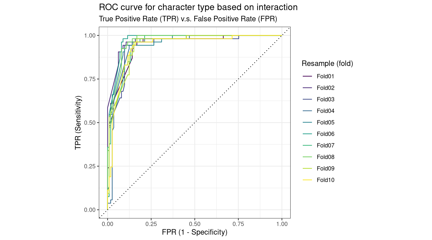
Figure 3: The machine learning model is far better at classifying characer types than random guessing.

Evaluating the model using the test data

From the 10-fold cross-validation training, we can see that this model is effective at classifying character type based on words used in interactions. To put this model to the test, we can use it to classify unseen data. Again, accuracy and ROC AUC will be used to evaluate model performance on the test data. A confusion matrix will also be plotted to illustrate performance: this matrix summarises model predictions versus the true values for observations in the test data.

# Fitting model to training data, evaluating performance on test data
char_type_last_fit <- last_fit(char_type_wf, char_type_split)
# Printing metrics for final fit
collect_metrics(char_type_last_fit)

# A tibble: 2 x 4
  .metric  .estimator .estimate .config             
  <chr>    <chr>          <dbl> <chr>               
1 accuracy binary         0.895 Preprocessor1_Model1
2 roc_auc  binary         0.952 Preprocessor1_Model1

# Plotting confusion matrix of testing data
collect_predictions(char_type_last_fit) %>%
  conf_mat(truth = char_type, estimate = .pred_class) %>%
  autoplot(type = "heatmap") +
  scale_fill_continuous() +
  labs(title = "Confusion matrix of lasso classification model performance on test subset",
       subtitle = "Sum of True Positives and False Positives for both classes: Computer and Person")

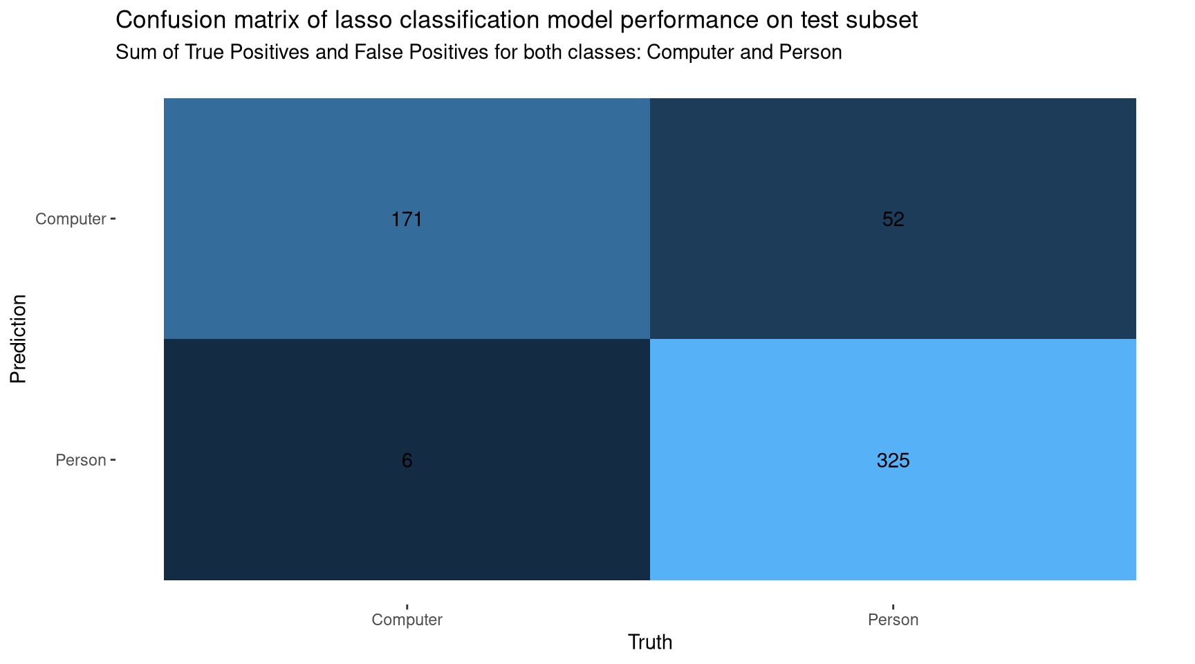
Figure 4: The model correctly classifies most observations in the test data.

Important words in the final model

The model is effective at classifying observations in the test data, with an accuracy of 89% and a ROC AUC of 95%. At this point, we may want to know more about how the model works. For example, which words had the largest impact on the model’s decision to classify a character type as “Computer” or “Person”? To see which words were important in the final model, we can extract the coefficient assigned to each word in the final fit, and plot the words with the highest values.

# Extracting model fit
char_type_workflow_fit <- pull_workflow_fit(char_type_last_fit$.workflow[[1]])

# Visualising the most important words for predicting whether a line was spoken
# by a Computer or Person character
tidy(char_type_workflow_fit) %>%
  filter(term != "Bias", term != "(Intercept)") %>%
  group_by(sign = estimate > 0) %>%
  slice_max(abs(estimate), n = 15) %>% 
  ungroup() %>%
  mutate(term = str_remove(term, "tfidf_interaction_"), # Tidying terms
         sign = ifelse(sign, "More likely from a Person",
                       "More likely a Computer")) %>%
  ggplot(aes(abs(estimate), fct_reorder(term, abs(estimate)), fill = sign)) +
  geom_col(show.legend = FALSE) +
  facet_wrap(~sign, scales = "free") +
  theme_classic() +
  scale_fill_viridis_d() +
  labs(titles = "Which words are more likely to be used by a Computer vs. Person character?",
       subtitle = "Importance assigned by lasso classification model, based lines spoken",
       x = "Coefficient from lasso regularised model", y = "Words")

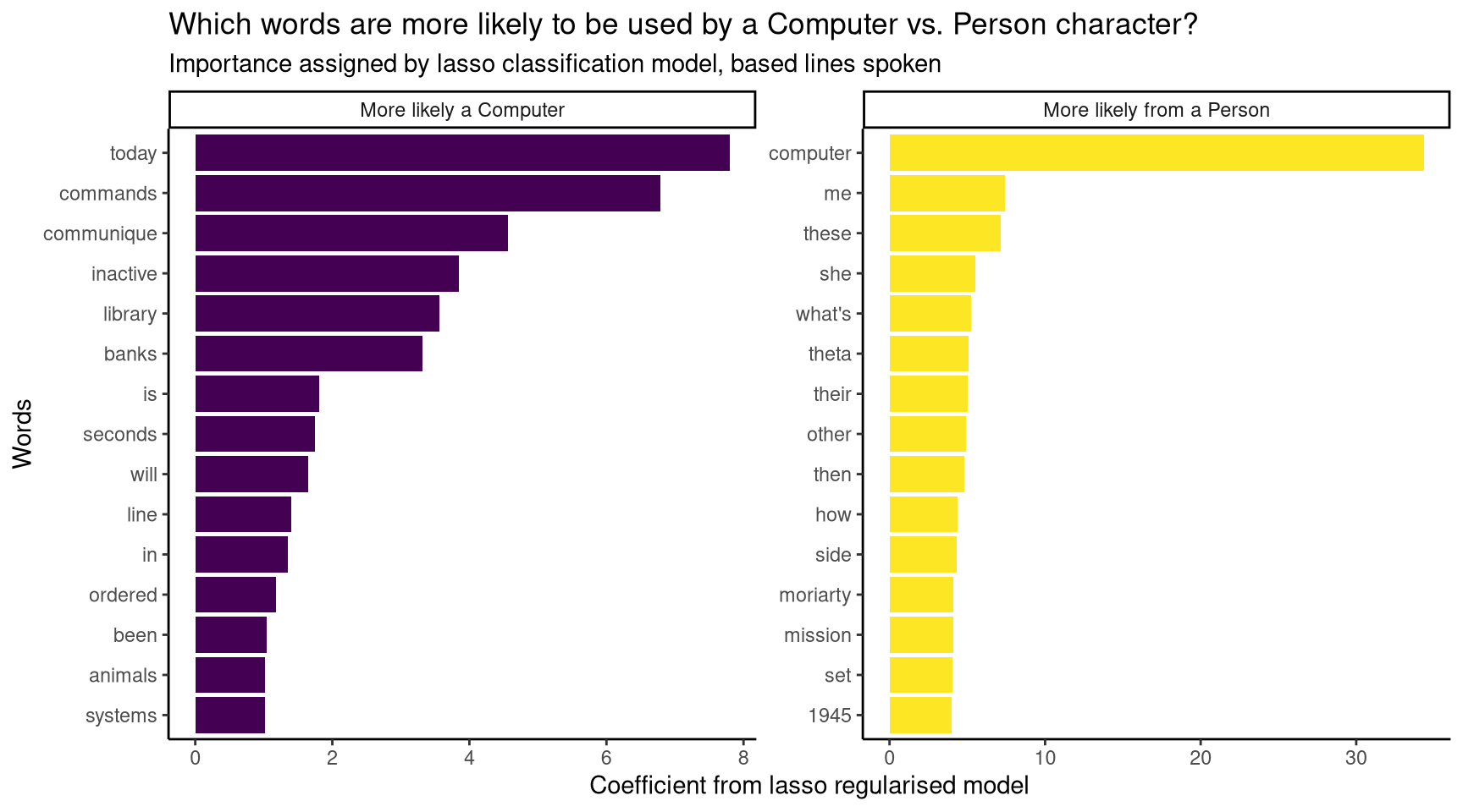
Figure 5: The model’s most important word for classifying Person characters was computer.

References

• Text Mining with R, Chapter 3 Analyzing word and document frequency: tf-idf
• Supervised Machine Learning for Text Analysis in R, Chapter 7 Classification