Setup
Loading the R libraries and data set.
# Loading libraries
library(geomtextpath) # For adding text to ggplot2 curves
library(tidytuesdayR) # For loading data set
library(ggbeeswarm) # For creating a beeswarm plot
library(tidyverse) # For the ggplot2, dplyr libraries
library(gganimate) # For plot animation
library(ggthemes) # For more ggplot2 themes
library(viridis) # For plot themes

# Loading data set
tt <- tt_load("2022-01-11")
    Downloading file 1 of 2: `colony.csv`
    Downloading file 2 of 2: `stressor.csv`
Data wrangling
In this section, the Bee Colony data is wrangled into two tidy sets:
tidied_colony_counts_overallcontains quarterly colony counts for the USAtidied_colony_counts_per_statecontains quarterly colony counts for various states within the USA
To create these sets, the original data is filtered to select for the appropriate states, and the “tidy_colony_data()” function is applied. These sets are tidy as each column is a variable, each row is an observation, and every cell has a single value. The types of observations in these data sets are:
Total colonies: Bee colonies countedLost: Bee colonies lostAdded: Bee colonies addedRenovated: Bee colonies renovated
# Creating subsets of the original bee colony data
colony_counts_overall <- tt$colony %>%
  filter(state == "United States")

colony_counts_per_state <- tt$colony %>%
  filter(state != "United States" & state != "Other states")

# Defining a function to tidy bee colony count data, which takes
# "messy_colony_data" as an argument
tidy_colony_data <- function(messy_colony_data){
  # Writing the result of the following piped steps to "tidied_colony_data"
  tidied_colony_data <- messy_colony_data %>%
    # Selecting variables
    select(year, colony_n, colony_lost, colony_added, colony_reno) %>%
    # Dropping rows with missing values
    drop_na() %>%
    # Changing columns to rows
    pivot_longer(!year, names_to = "type", values_to = "count") %>%
    # Setting "type" as a factor variable
    mutate(type = factor(type)) %>%
    # Recoding the levels of the "type" factor
    mutate(type = fct_recode(type,
                             "Total colonies" = "colony_n",
                             "Lost" = "colony_lost",
                             "Added" = "colony_added",
                             "Renovated" = "colony_reno")) %>%
    # Reordering "type" factor levels
    mutate(type = fct_relevel(type,
                              "Total colonies", "Lost", "Added", "Renovated"))
  # Returning "tidied_colony_data"
  return(tidied_colony_data)
}

# Using this function to tidy the subsets
tidied_colony_counts_overall <- tidy_colony_data(colony_counts_overall)

tidied_colony_counts_per_state <- tidy_colony_data(colony_counts_per_state)

# Printing a summary of the subsets before tidying...
colony_counts_overall
# A tibble: 26 x 10
    year months  state colony_n colony_max colony_lost colony_lost_pct
   <dbl> <chr>   <chr>    <dbl>      <dbl>       <dbl>           <dbl>
 1  2015 Januar~ Unit~  2824610         NA      500020              18
 2  2015 April-~ Unit~  2849500         NA      352860              12
 3  2015 July-S~ Unit~  3132880         NA      457100              15
 4  2015 Octobe~ Unit~  2874760         NA      412380              14
 5  2016 Januar~ Unit~  2594590         NA      428800              17
 6  2016 April-~ Unit~  2801470         NA      329820              12
 7  2016 July-S~ Unit~  3181180         NA      397290              12
 8  2016 Octobe~ Unit~  3032060         NA      502350              17
 9  2017 Januar~ Unit~  2615590         NA      361850              14
10  2017 April-~ Unit~  2886030         NA      225680               8
# ... with 16 more rows, and 3 more variables: colony_added <dbl>,
#   colony_reno <dbl>, colony_reno_pct <dbl>
colony_counts_per_state
# A tibble: 1,196 x 10
    year months  state colony_n colony_max colony_lost colony_lost_pct
   <dbl> <chr>   <chr>    <dbl>      <dbl>       <dbl>           <dbl>
 1  2015 Januar~ Alab~     7000       7000        1800              26
 2  2015 Januar~ Ariz~    35000      35000        4600              13
 3  2015 Januar~ Arka~    13000      14000        1500              11
 4  2015 Januar~ Cali~  1440000    1690000      255000              15
 5  2015 Januar~ Colo~     3500      12500        1500              12
 6  2015 Januar~ Conn~     3900       3900         870              22
 7  2015 Januar~ Flor~   305000     315000       42000              13
 8  2015 Januar~ Geor~   104000     105000       14500              14
 9  2015 Januar~ Hawa~    10500      10500         380               4
10  2015 Januar~ Idaho    81000      88000        3700               4
# ... with 1,186 more rows, and 3 more variables: colony_added <dbl>,
#   colony_reno <dbl>, colony_reno_pct <dbl>
# ...and after tidying
tidied_colony_counts_overall
# A tibble: 100 x 3
    year type             count
   <dbl> <fct>            <dbl>
 1  2015 Total colonies 2824610
 2  2015 Lost            500020
 3  2015 Added           546980
 4  2015 Renovated       270530
 5  2015 Total colonies 2849500
 6  2015 Lost            352860
 7  2015 Added           661860
 8  2015 Renovated       692850
 9  2015 Total colonies 3132880
10  2015 Lost            457100
# ... with 90 more rows
tidied_colony_counts_per_state
# A tibble: 4,208 x 3
    year type           count
   <dbl> <fct>          <dbl>
 1  2015 Total colonies  7000
 2  2015 Lost            1800
 3  2015 Added           2800
 4  2015 Renovated        250
 5  2015 Total colonies 35000
 6  2015 Lost            4600
 7  2015 Added           3400
 8  2015 Renovated       2100
 9  2015 Total colonies 13000
10  2015 Lost            1500
# ... with 4,198 more rows
Plotting Bee Colony observations using {ggbeeswarm}
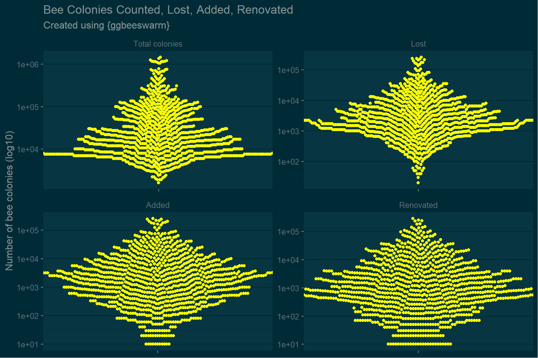
The first graph plots a point for each type of observation using geom_beeswarm().
# Plotting Bee Colony observations using geom_beeswarm() from {ggbeeswarm}
tidied_colony_counts_per_state %>%
  ggplot(aes(x = type, y = count)) +
  geom_beeswarm(cex = 4, colour = "yellow") +
  scale_y_log10() +
  theme_solarized_2(light = FALSE) +
  facet_wrap(~type, scales = "free") +
  theme(legend.position="none", axis.text.x = element_blank()) +
  labs(title = "Bee Colonies Counted, Lost, Added, Renovated",
       subtitle = "Created using {ggbeeswarm}",
       x = NULL, y = "Number of bee colonies (log10)",
       fill = NULL)

Figure 1: Scatter plots of bee colony observations. This plot has a point for each observation. Points are jittered to reduce overplotting.
Animating Bee Colony observations over time
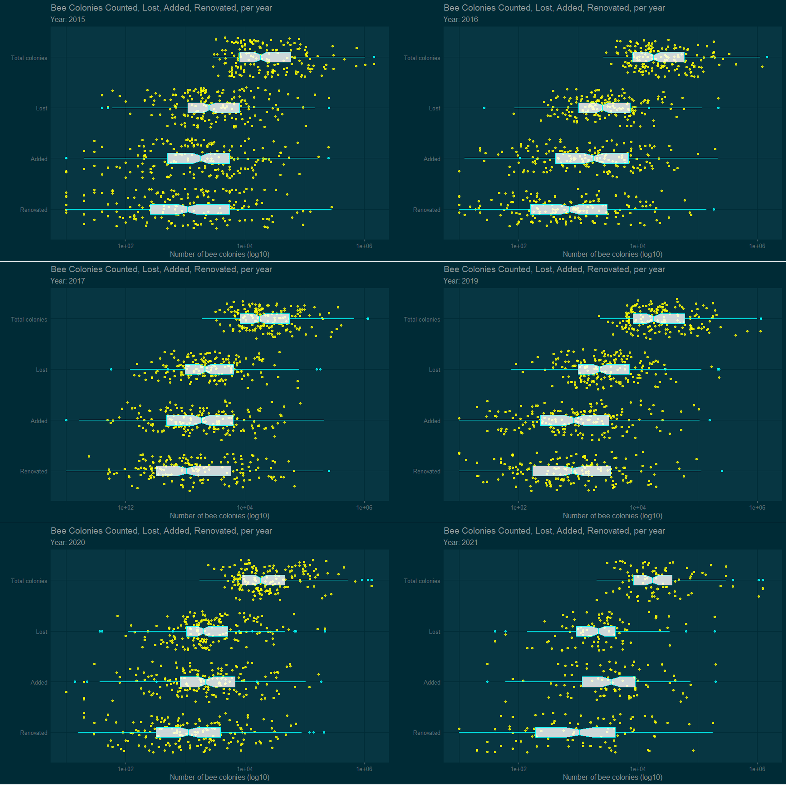
While the previous plot is thematically appropriate, it could be better. This graph plots the same points over time in an animation, with the year plotted given in the subtitle. This graph uses standard {ggplot2} jittered points, as well as a box plot to illustrate the distribution of the points. These box plots have notches, showing 95% confidence intervals for the median. Distributions with notches that do not overlap differ significantly.
# Defining an animation showing bee colony counts over time
p <- tidied_colony_counts_per_state %>%
  ggplot(aes(x = count, y = fct_reorder(type, count))) +
  geom_jitter(color = "yellow", alpha = 0.8) +
  geom_boxplot(width = 0.2, alpha = 0.8, notch = TRUE, colour = "cyan") +
  scale_x_log10() +
  theme_solarized_2(light = FALSE) +
  theme(legend.position="none", axis.ticks.y = element_blank(),
        axis.line.y = element_blank()) +
  transition_time(as.integer(year)) +
  labs(title = "Bee Colonies Counted, Lost, Added, Renovated, per year",
       subtitle = "Year: {frame_time}",
       x = "Number of bee colonies (log10)", y = NULL)

# Rendering the animation as a .gif
animate(p, nframes = 180, start_pause = 20,  end_pause = 20,
        renderer = magick_renderer())

Figure 2: Animation showing bee colony counts from 2015 to 2021.
Plotting the distribution of different Bee Colony observation types
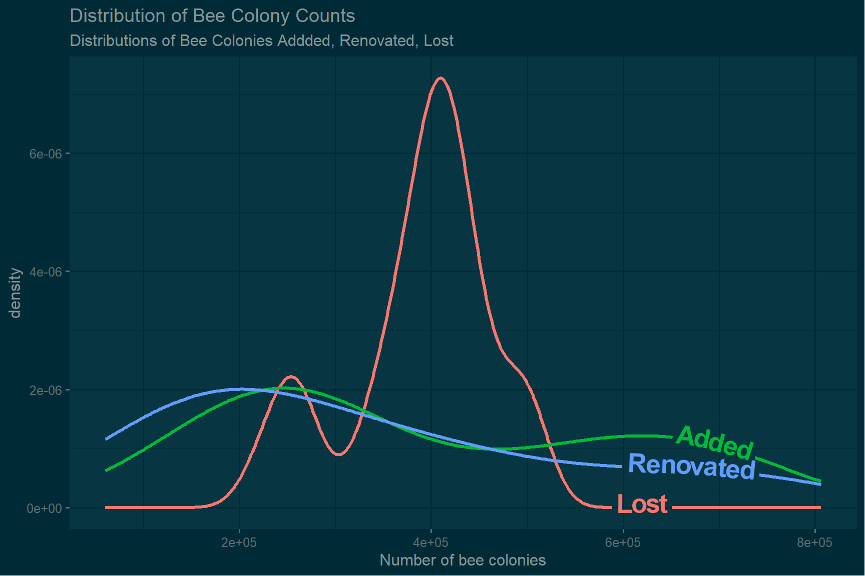
From the previous plot, we can see that the Added and Renovated variables have similar distributions based on their box plots. Distributions can also be visualised using density plots. In this graph, the distribution of different types of observation in the data set are plotted.
# Creating a density plot for different observation types
tidied_colony_counts_overall %>%
  filter(type != "Total colonies") %>%
  ggplot(aes(x = count, colour = type, label = type)) +
  geom_textdensity(size = 7, fontface = 2, hjust = 0.89, vjust = 0.3,
                   linewidth = 1.2) +
  theme_solarized_2(light = FALSE) +
  theme(legend.position = "none") +
  labs(title = "Distribution of Bee Colony Counts",
       subtitle = "Distributions of Bee Colonies Addded, Renovated, Lost",
       x = "Number of bee colonies")

Figure 3: A density plot, giving the distribution of various observations. Of the three types of observation plotted, Added and Renovated are the most similar.