Introduction
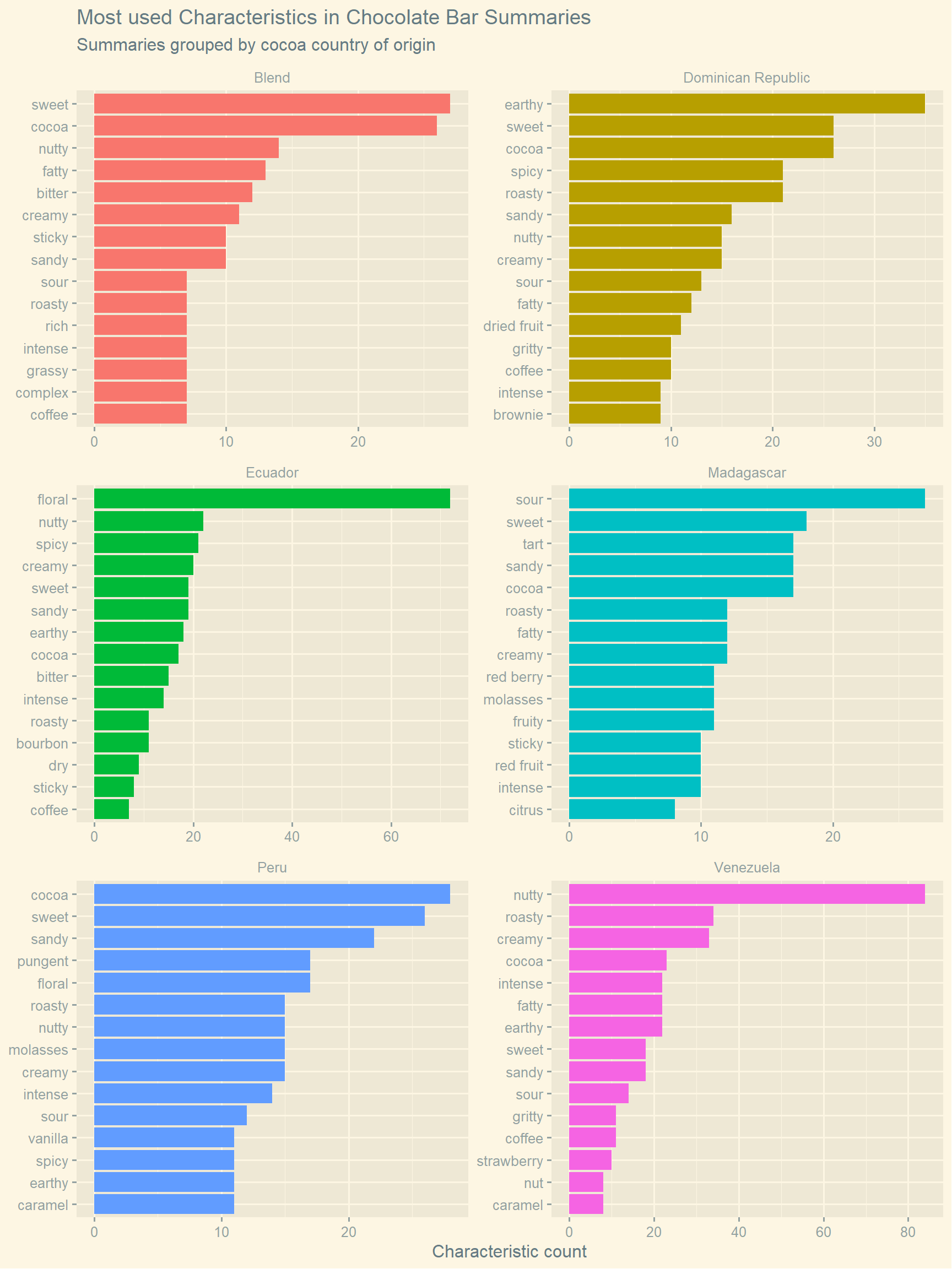
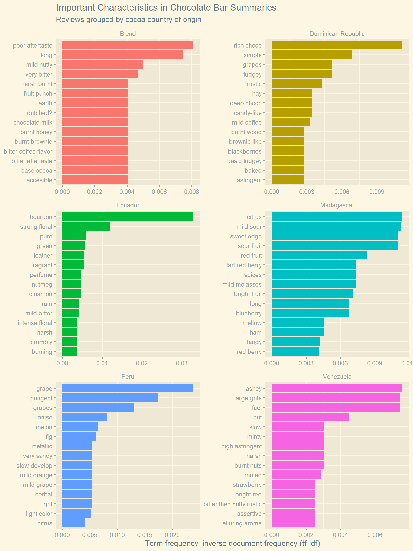
In this post, memorable characteristics of chocolate bars are plotted. These characteristics relate to anything about the bars, e.g. texture, flavour, overall opinion. This data set includes the country of cocoa bean origin for each chocolate bar, including “blend” for bars with multiple beans. To create these plots, the data set is filtered to select the six countries of origin with the most chocolate bar characteristics.
The first plot lists the top fifteen most used characteristics for bars from each country. The countries of origin cannot be distinguished based on this plot, most of the characteristics listed can be applied to all the chocolate bars in the data set. “Sweet” is listed in every plot, for example. To find characteristics that are unique or important to chocolate from each country, term frequency–inverse document frequency (tf-idf) can be used to select characteristics, instead of number of occurrences alone. In this case, the characteristics associated with each country are treated as separate documents. The second plot lists the top fifteen most characteristics for the same chocolate bars using tf-idf. From this plot, we can see characteristics that are often associated with one group of chocolate bars, but not the other groups. For example, chocolate bars made using a blend of beans are the most likely to list “poor after taste” as a characteristics, whereas “grape” is a characteristic most likely associated with Peruvian chocolate bars.
Setup
Loading the R libraries and data set.
# Loading libraries
library(tidytuesdayR)
library(tidyverse)
library(ggthemes)
library(tidytext)

# Loading data
tt <- tt_load("2022-01-18")
Downloading file 1 of 1: `chocolate.csv`Data wrangling
# Counting how many times each characteristic is used
country_characteristics <- tt$chocolate %>%
  unnest_tokens(memorable_characteristic,
                most_memorable_characteristics, token = "regex",
                pattern = ",", to_lower = TRUE) %>%
  mutate(memorable_characteristic = str_squish(memorable_characteristic)) %>%
  count(country_of_bean_origin, memorable_characteristic, sort = TRUE)

# Counting the total number of characteristics used for each country of origin
total_country_characteristics <- country_characteristics %>%
  group_by(country_of_bean_origin) %>%
  summarise(total = sum(n))

# Joining these data frames
country_characteristics <- left_join(country_characteristics,
                                     total_country_characteristics,
                                     by = "country_of_bean_origin")

# Finding the six countries of origin with the most characteristics
top_countries <- total_country_characteristics %>%
  slice_max(n = 6, order_by = total) %>%
  select(country_of_bean_origin)

# Filtering the data
country_characteristics <- country_characteristics %>%
  filter(country_of_bean_origin %in% top_countries$country_of_bean_origin) %>%
  select(country_of_bean_origin, memorable_characteristic, n, total)

# Adding tf-idf
country_characteristics <- country_characteristics %>%
  bind_tf_idf(memorable_characteristic,
              country_of_bean_origin, n)

# Printing a summary of the data frame
country_characteristics
# A tibble: 1,233 x 7
   country_of_bean_~ memorable_charac~     n total     tf   idf tf_idf
   <chr>             <chr>             <int> <int>  <dbl> <dbl>  <dbl>
 1 Venezuela         nutty                84   722 0.116      0      0
 2 Ecuador           floral               72   600 0.12       0      0
 3 Dominican Republ~ earthy               35   641 0.0546     0      0
 4 Venezuela         roasty               34   722 0.0471     0      0
 5 Venezuela         creamy               33   722 0.0457     0      0
 6 Peru              cocoa                28   678 0.0413     0      0
 7 Blend             sweet                27   443 0.0609     0      0
 8 Madagascar        sour                 27   485 0.0557     0      0
 9 Blend             cocoa                26   443 0.0587     0      0
10 Dominican Republ~ cocoa                26   641 0.0406     0      0
# ... with 1,223 more rows
Plotting the most used characteristics in the chocolate bar summaries
# Plotting the most used characteristics in the chocolate bar summaries
country_characteristics %>%
  group_by(country_of_bean_origin) %>%
  slice_max(n, n = 15, with_ties = FALSE) %>%
  ungroup() %>%
  mutate(country_of_bean_origin = as.factor(country_of_bean_origin),
         memorable_characteristic = reorder_within(memorable_characteristic,
                                                   n,
                                                   country_of_bean_origin)) %>%
  ggplot(aes(n, memorable_characteristic, fill = country_of_bean_origin)) +
  geom_col(show.legend = FALSE) +
  scale_y_reordered() +
  theme_solarized_2() +
  facet_wrap(~country_of_bean_origin, ncol = 2, scales = "free") +
  labs(title = "Most used Characteristics in Chocolate Bar Summaries",
       subtitle = "Summaries grouped by cocoa country of origin",
       x = "Characteristic count", y = NULL)

Figure 1: Characteristics that are most used to describe chocolate bars made using different cocoa beans are plotted.
Plotting the most important characteristics in the chocolate bar summaries
# Plotting the most important characteristics in the chocolate bar summaries
country_characteristics %>%
  group_by(country_of_bean_origin) %>%
  slice_max(tf_idf, n = 15, with_ties = FALSE) %>%
  ungroup() %>%
  mutate(country_of_bean_origin = as.factor(country_of_bean_origin),
         memorable_characteristic = reorder_within(memorable_characteristic,
                                                   tf_idf,
                                                   country_of_bean_origin)) %>%
  ggplot(aes(tf_idf, memorable_characteristic, fill = country_of_bean_origin)) +
  geom_col(show.legend = FALSE) +
  scale_y_reordered() +
  theme_solarized_2() +
  facet_wrap(~country_of_bean_origin, ncol = 2, scales = "free") +
  labs(title = "Important Characteristics in Chocolate Bar Summaries",
       subtitle = "Reviews grouped by cocoa country of origin",
       x = "Term frequency–inverse document frequency (tf-idf)", y = NULL)

Figure 2: Characteristics that are often used to describe chocolate bars made using cocoa from a given country, but not for other chocolate bars, are plotted.
References