Introduction
In this post, the European Flights data set is used to illustrate defining a function in R and applying it to a data frame using map functions from {purrr}. The full source for this blog post is available on GitHub.
Setup
Loading the R libraries and data set.
# Loading libraries
library(tidytuesdayR)
library(tidyverse)
library(tidytext)
library(ggthemes)

# Loading data
tt <- tt_load("2022-07-12")
Downloading file 1 of 1: `flights.csv`Defining a function to tidy flight types and applying it with purrr::map
In this section, we want to tidy the different types of flight in the data set by increasing the number of rows and decreasing the number of columns. For a given airport on a given day, instead of having multiple columns/variables for arrivals, departures and total number of flights, we want to have one column describing the flight type (e.g. arrival or departure) and one column with the value of that flight type/number of flights. This will give the data set a tidy structure.
# Printing a summary of the flights data frame
tt$flights
# A tibble: 688,099 × 14
YEAR MONTH_NUM MONTH_MON FLT_DATE APT_ICAO APT_NAME
<dbl> <chr> <chr> <dttm> <chr> <chr>
1 2016 01 JAN 2016-01-01 00:00:00 EBAW Antwerp
2 2016 01 JAN 2016-01-01 00:00:00 EBBR Brussels
3 2016 01 JAN 2016-01-01 00:00:00 EBCI Charleroi
4 2016 01 JAN 2016-01-01 00:00:00 EBLG Liège
5 2016 01 JAN 2016-01-01 00:00:00 EBOS Ostend-Brug…
6 2016 01 JAN 2016-01-01 00:00:00 EDDB Berlin - Br…
7 2016 01 JAN 2016-01-01 00:00:00 EDDC Dresden
8 2016 01 JAN 2016-01-01 00:00:00 EDDE Erfurt
9 2016 01 JAN 2016-01-01 00:00:00 EDDF Frankfurt
10 2016 01 JAN 2016-01-01 00:00:00 EDDG Muenster-Os…
# … with 688,089 more rows, and 8 more variables: STATE_NAME <chr>,
# FLT_DEP_1 <dbl>, FLT_ARR_1 <dbl>, FLT_TOT_1 <dbl>,
# FLT_DEP_IFR_2 <dbl>, FLT_ARR_IFR_2 <dbl>, FLT_TOT_IFR_2 <dbl>,
# `Pivot Label` <chr># Printing a summary of the shape of the data frame
paste("tt$flights has", nrow(tt$flights), "rows and", ncol(tt$flights),
"columns.")[1] "tt$flights has 688099 rows and 14 columns."# Defining a function to tidy the flights data set
tidy_flights_per_airport <- function(input_flight_type){
tt$flights %>%
# Selecting columns, including the column with the name "input_flight_type"
## "all_of()" is used for error handling: if a column with the name matching
## "input_flight_type" is not available in tt$flights, the function will return an error
select(FLT_DATE, APT_NAME, all_of(input_flight_type)) %>%
# Adding a "flight_type" column, with "input_flight_type" as a string for each row
mutate(flight_type = as.character(input_flight_type)) %>%
# Renaming the input "input_flight_type" column to "number_of_flights"
rename("number_of_flights" = input_flight_type)
}
# Selecting column names with flight types (arrivals, departures, total flights)
flight_types <- colnames(tt$flights)[8:13]
# Printing the flight types
flight_types[1] "FLT_DEP_1" "FLT_ARR_1" "FLT_TOT_1" "FLT_DEP_IFR_2"
[5] "FLT_ARR_IFR_2" "FLT_TOT_IFR_2"# Applying the tidying function to the flight types vector using purrr::map()
tidy_flights_list <- map(flight_types, tidy_flights_per_airport)Binding the tidied flight type rows into a data frame with purrr::map_df
Using the map function in the previous section returned a list of tidied flight types: the “tidy_flights_per_airport()” function was applied to each item in “flight_types” individually, and the resulting tidied flight type was added to “tidy_flights_list”. In this section, the “rbind()” function is applied to “tidy_flights_list” to create a single data frame with all of the tidied flight types.
# Binding the tidy version of each flight type by row using purrr::map_df
tidy_flights <- map_df(tidy_flights_list, rbind)

# Printing a summary of the tidy flights data frame
tidy_flights
# A tibble: 4,128,594 × 4
FLT_DATE APT_NAME number_of_fligh… flight_type
<dttm> <chr> <dbl> <chr>
1 2016-01-01 00:00:00 Antwerp 4 FLT_DEP_1
2 2016-01-01 00:00:00 Brussels 174 FLT_DEP_1
3 2016-01-01 00:00:00 Charleroi 45 FLT_DEP_1
4 2016-01-01 00:00:00 Liège 6 FLT_DEP_1
5 2016-01-01 00:00:00 Ostend-Bruges 7 FLT_DEP_1
6 2016-01-01 00:00:00 Berlin - Brandenb… 98 FLT_DEP_1
7 2016-01-01 00:00:00 Dresden 18 FLT_DEP_1
8 2016-01-01 00:00:00 Erfurt 1 FLT_DEP_1
9 2016-01-01 00:00:00 Frankfurt 401 FLT_DEP_1
10 2016-01-01 00:00:00 Muenster-Osnabrue… 3 FLT_DEP_1
# … with 4,128,584 more rows# Printing a summary of the shape of the data frame
paste("tidy_flights has", nrow(tidy_flights), "rows and", ncol(tidy_flights),
"columns.")[1] "tidy_flights has 4128594 rows and 4 columns."The tidy_flights data frame is now in a tidy format.
Plotting the distribution of arrivals and departures across the top six airports
## Selecting the top 6 airports by total number of flights on the latest flight
## date
top_airports <- tidy_flights %>%
  filter(flight_type == "FLT_TOT_1") %>%
  filter(FLT_DATE == max(FLT_DATE)) %>%
  slice_max(order_by = number_of_flights, n = 6)

# Changing "flight_type" to a factor with descriptive levels
tidy_flights$flight_type <- as.factor(tidy_flights$flight_type)
levels(tidy_flights$flight_type) <- c("Arrivals", "Arrivals (Airport Operator)",
  "Departures", "Departures (Airport Operator)", "Total", "Total (Airport Operator")

# Plotting the distribution of arrivals and departures for the top airports
tidy_flights %>%
  filter(APT_NAME %in% top_airports$APT_NAME) %>%
  filter(flight_type %in% c("Arrivals", "Departures")) %>%
  ggplot(aes(x = APT_NAME, y = number_of_flights, colour = flight_type)) +
  geom_boxplot() +
  theme_solarized() +
  theme(axis.text.x = element_text(angle = 45, hjust = 1)) +
  scale_colour_discrete() +
  labs(title = "Distribution of daily arrivals and depatures across six airports",
    x = "Airport", y = "Flights", colour = "Flight type")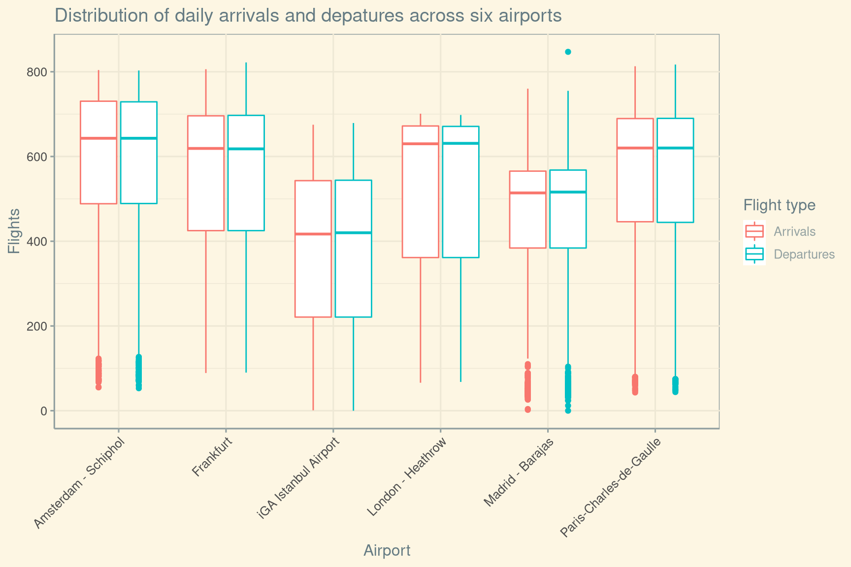
Figure 1: Box plots of daily arrival and depature distribution across top six airports.
See also